Linear programming:

Linear programming is a fundamental optimization technique that been used from many years in science and math fields.

Linear programming is a way of achieving the best outcome, such as maximum profit or minimum cost, using a mathematical model represented by linear relationships.

Importance of Linear programming

Most business problems don't have straightforward solutions. Decision making requires leaders to consider many variables and constraints, and this makes manual solutions difficult to achieve. Linear programming software helps leaders solve complex problems quickly and easily by providing an optimal solution.

Importance in recent years due to its application in coding and Artificial

Intelligence (AI), and as a form of linear regression in data science.

Application of linear programming:

Manufacturing : Mainly faced by production companies, this type of problem involves solving for making the maximum profit or minimum cost given various constraints like labor, output units, and machine runtime
Transportation : This type of problem includes finding the right transportation solutions given the constraints of cost and time.
Financial planning: LP can be used in financial planning to determine the optimal allocation of resources to maximize profits while minimizing costs and risks.
Agriculture: Linear programming can be used in agriculture to optimize crop yields, determine the best crop rotation, and allocate resources such as land, water, and fertilizers.
Energy: Linear programming is used in the energy sector to optimize the distribution and production of electricity and other forms of energy, as well as to plan the optimal use of renewable energy sources.

Components of Linear Programming

1. Decision Variables

These are the unknown quantities in an optimization problem that need to be solved. For example, in the case of a company wanting to decide its production levels for the next twelve months, given various constraints, the production levels become the decision variables.

2. Constraints

Constraints are the limitations one needs to consider while solving a given problem. For example, constraints can be regarding resources such as time, cost, and so on.

3. Objective Functions

Objective functions are the real-valued functions that need to be optimized for either minimum or maximum output given a set of constraints.

5. Non-Negativity Restriction

The decision variables should always take non-negative values, i.e. they should be greater than or equal to 0.

Methods to Solve Linear Programming Problems

Graphical method
Simplex method

Graphical Method

This method is used to solve a two-variable linear program. If you have only two decision variables, you should use the graphical method to find the optimal solution.

A graphical method involves formulating a set of linear inequalities subject to the constraints. Then the inequalities are plotted on an X-Y plane. Once we have plotted all the inequalities on a graph the intersecting region gives us a feasible region. The feasible region explains what all values our model can take. And it also gives us the best solution.

Example :

Suppose we have to maximize Z = 2x + 5y.

The constraints are x + 4y ≤ 24, 3x + y ≤ 21 and x + y ≤ 9

where, x ≥ 0 and y ≥ 0.

To solve this problem using the graphical method the steps are as follows.

Step 1: Write all inequality constraints in the form of equations.

x + 4y = 24

3x + y = 21

x + y = 9

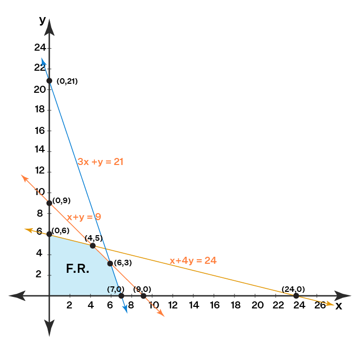
Step 2: Plot these lines on a graph by identifying test points.

x + 4y = 24 is a line passing through (0, 6) and (24, 0).

[By substituting x = 0 the point (0, 6) is obtained. Similarly, when y = 0 the point (24, 0) is determined.]

3x + y = 21 passes through (0, 21) and (7, 0).

x + y = 9 passes through (9, 0) and (0, 9).

Step 3: Identify the feasible region.

Any point that lies on or below the line x + 4y = 24 will satisfy the constraint x + 4y ≤ 24.

Similarly, a point that lies on or below 3x + y = 21 satisfies 3x + y ≤ 21.

Also, a point lying on or below the line x + y = 9 satisfies x + y ≤ 9.

The feasible region is represented by OABCD as it satisfies all the above-mentioned three restrictions.

Step 4: Determine the coordinates of the corner points.

The corner points are the vertices of the feasible region.

O = (0, 0)

A = (7, 0)

B = (6, 3). B is the intersection of the two lines 3x + y = 21 and x + y = 9. Thus,

by substituting y = 9 - x in 3x + y = 21 we can determine the point of intersection.

C = (4, 5) formed by the intersection of x + 4y = 24 and x + y = 9

D = (0, 6)

Linear Programming by Graphical Method

Step 5: Substitute each corner point in the objective function.

The point that gives the greatest (maximizing) or smallest (minimizing) value of the objective function will be the optimal point.

Corner Points	Z = 2x + 5y
O = (0, 0)	0
A = (7, 0)	14
B = (6, 3)	27
C = (4, 5)	33
D = (0, 6)	30

33 is the maximum value of Z and it occurs at C. Thus, the solution is x = 4 and y = 5.

Simplex Method

The simplex method in linear programming can be applied to problems with two or more decision variables.

Example:

objective function Z = 40 $x_{1}$ + 30 $x_{2}$ needs to be maximized and the constraints are given as follows:

$x_{1}$ + $x_{2}$ ≤ 12

2 $x_{1}$ + $x_{2}$ ≤ 16

$x_{1}$ ≥ 0, $x_{2}$ ≥ 0

Step 1: Add another variable, known as the slack variable, to convert the inequalities into equations. Also, rewrite the objective function as an equation.

- 40 $x_{1}$ - 30 $x_{2}$ + Z = 0

$x_{1}$ + $x_{2}$ + $y_{1}$ =12

2 $x_{1}$ + $x_{2}$ + $y_{2}$ =16

$y_{1}$ and $y_{2}$ are the slack variables.

Step 2: Construct the initial simplex matrix as follows:

$[\begin{matrix} x_{1} & x_{2} & y_{1} & y_{2} & Z \\ 1 & 1 & 1 & 0 & 0 & 12 \\ 2 & 1 & 0 & 1 & 0 & 16 \\ - 40 & - 30 & 0 & 0 & 1 & 0 \end{matrix}]$

Step 3: Identify the column with the highest negative entry.

This is called the pivot column. As -40 is the highest negative entry, thus, column 1 will be the pivot column.

Step 4: Divide the entries in the rightmost column by the entries in the pivot column. We exclude the entries in the bottom-most row.

12 / 1 = 12

16 / 2 = 8

The row containing the smallest quotient is identified to get the pivot row.

As 8 is the smaller quotient as compared to 12 thus, row 2 becomes the pivot row.

The intersection of the pivot row and the pivot column gives the pivot element.

Thus, pivot element = 2.

Step 5: With the help of the pivot element perform pivoting, using matrix properties,

to make all other entries in the pivot column 0.

Using the elementary operations divide row 2 by 2 ( $R_{2}$ / 2)

$[\begin{matrix} x_{1} & x_{2} & y_{1} & y_{2} & Z \\ 1 & 1 & 1 & 0 & 0 & 12 \\ 1 & 1 / 2 & 0 & 1 / 2 & 0 & 8 \\ - 40 & - 30 & 0 & 0 & 1 & 0 \end{matrix}]$

Now apply $R_{1}$ = $R_{1}$ - $R_{2}$

$[\begin{matrix} x_{1} & x_{2} & y_{1} & y_{2} & Z \\ 0 & 1 / 2 & 1 & - 1 / 2 & 0 & 4 \\ 1 & 1 / 2 & 0 & 1 / 2 & 0 & 8 \\ - 40 & - 30 & 0 & 0 & 1 & 0 \end{matrix}]$

Finally $R_{3}$ = $R_{3}$ + 40 $R_{2}$ to get the required matrix.

$[\begin{matrix} x_{1} & x_{2} & y_{1} & y_{2} & Z \\ 0 & 1 / 2 & 1 & - 1 / 2 & 0 & 4 \\ 1 & 1 / 2 & 0 & 1 / 2 & 0 & 8 \\ 0 & - 10 & 0 & 20 & 1 & 320 \end{matrix}]$

Step 6: Check if the bottom-most row has negative entries. If no, then the optimal solution has been determined. If yes, then go back to step 3 and repeat the process. -10 is a negative entry in the matrix thus, the process needs to be repeated. We get the following matrix.

$[\begin{matrix} x_{1} & x_{2} & y_{1} & y_{2} & Z \\ 0 & 1 & 2 & - 1 & 0 & 8 \\ 1 & 0 & - 1 & 1 & 0 & 4 \\ 0 & 0 & 20 & 10 & 1 & 400 \end{matrix}]$

Writing the bottom row in the form of an equation we get Z = 400 - 20 $y_{1}$ - 10 $y_{2}$ . Thus,

400 is the highest value that Z can achieve when both $y_{1}$ and $y_{2}$ are 0.

, when $x_{1}$ = 4 and $x_{2}$ = 8 then value of Z = 400

Thus, $x_{1}$ = 4 and $x_{2}$ = 8 are the optimal points and the solution to our linear

programming problem.

Search This Blog

Linear Programming Problems(LPP)

linear programming explaination